Frost Days in the Pyrenees: 1980 vs 2023 Comparison
This notebook demonstrates how to compare frost days between two distinct years (1980 and 2023) using ERA5 reanalysis data in its native GRIB format. Using the earthkit-climate package, we will compute the Frost Days (FD) index for the Aragonese Pyrenees and visualize the difference in frost occurrences.
Prerequisites & Data Access
To run this notebook, you must have an account on the Copernicus Climate Data Store (CDS).
CDS API Configuration
Because earthkit retrieves ERA5 data via the cdsapi, you need to configure your API access. Instead of manual local configuration, we recommend following the official guide to ensure your setup is always up to date:
What is the Frost Days (FD) Index?
The Frost Days index is defined as the number of days in a year where the daily minimum temperature (\(T_{min}\)) falls below 0°C. It is a key indicator for agriculture, hydrology, and biodiversity in high-mountain ecosystems.
1. Setup and Study Area
First, we import the necessary libraries and define our coordinates for the Aragonese Pyrenees (Bounding Box).
[1]:
import earthkit.data as ekd
import earthkit.plots as ekp
import earthkit.transforms as ekt
import numpy as np

import earthkit.climate as ekc
2. Data Acquisition (ERA5)
We use the Copernicus Climate Data Store (CDS) API to download hourly 2m temperature data. You can find the official dataset entry here:
We download data for the peak frost months (January-March and October-December) for both 1980 and 2023 for our study area.
[2]:
# 1. Define the study area [North, West, South, East]
# Coordinates for the Aragonese Pyrenees
PYRENEES_AREA = [43, -1, 42, 0.8]

print("Requesting data from CDS... (this might take a few minutes)")

# 2. Retrieve and open 1980 data (The Baseline)
data_1980 = ekd.from_source(
    "cds",
    "reanalysis-era5-single-levels",
    request={
        "variable": "2m_temperature",
        "product_type": "reanalysis",
        "year": "1980",
        "month": [f"{i:02d}" for i in range(1, 13)],
        "day": [f"{i:02d}" for i in range(1, 32)],
        "time": [f"{i:02d}:00" for i in range(24)],
        "area": PYRENEES_AREA,
        "format": "grib",
    },
)

# 4. Retrieve and open 2023 data (The Comparison)
data_2023 = ekd.from_source(
    "cds",
    "reanalysis-era5-single-levels",
    request={
        "variable": "2m_temperature",
        "product_type": "reanalysis",
        "year": "2023",
        "month": [f"{i:02d}" for i in range(1, 13)],
        "day": [f"{i:02d}" for i in range(1, 32)],
        "time": [f"{i:02d}:00" for i in range(24)],
        "area": PYRENEES_AREA,
        "format": "grib",
    },
)

print("Data successfully loaded into earthkit objects!")
Requesting data from CDS... (this might take a few minutes)
2026-06-02 16:58:32,719 INFO [2025-12-11T00:00:00] Please note that a dedicated catalogue entry for this dataset, post-processed and stored in Analysis Ready Cloud Optimized (ARCO) format (Zarr), is available for optimised time-series retrievals (i.e. for retrieving data from selected variables for a single point over an extended period of time in an efficient way). You can discover it [here](https://cds.climate.copernicus.eu/datasets/reanalysis-era5-single-levels-timeseries?tab=overview)
INFO:ecmwf.datastores.legacy_client:[2025-12-11T00:00:00] Please note that a dedicated catalogue entry for this dataset, post-processed and stored in Analysis Ready Cloud Optimized (ARCO) format (Zarr), is available for optimised time-series retrievals (i.e. for retrieving data from selected variables for a single point over an extended period of time in an efficient way). You can discover it [here](https://cds.climate.copernicus.eu/datasets/reanalysis-era5-single-levels-timeseries?tab=overview)
2026-06-02 16:58:32,719 INFO Request ID is 4061e53d-f5c1-49d5-ab43-be74ea806412
INFO:ecmwf.datastores.legacy_client:Request ID is 4061e53d-f5c1-49d5-ab43-be74ea806412
2026-06-02 16:58:32,811 INFO status has been updated to accepted
INFO:ecmwf.datastores.legacy_client:status has been updated to accepted
2026-06-02 16:58:43,137 INFO status has been updated to running
INFO:ecmwf.datastores.legacy_client:status has been updated to running
2026-06-02 17:10:56,194 INFO status has been updated to successful
INFO:ecmwf.datastores.legacy_client:status has been updated to successful
2026-06-02 17:10:58,581 INFO [2025-12-11T00:00:00] Please note that a dedicated catalogue entry for this dataset, post-processed and stored in Analysis Ready Cloud Optimized (ARCO) format (Zarr), is available for optimised time-series retrievals (i.e. for retrieving data from selected variables for a single point over an extended period of time in an efficient way). You can discover it [here](https://cds.climate.copernicus.eu/datasets/reanalysis-era5-single-levels-timeseries?tab=overview)
INFO:ecmwf.datastores.legacy_client:[2025-12-11T00:00:00] Please note that a dedicated catalogue entry for this dataset, post-processed and stored in Analysis Ready Cloud Optimized (ARCO) format (Zarr), is available for optimised time-series retrievals (i.e. for retrieving data from selected variables for a single point over an extended period of time in an efficient way). You can discover it [here](https://cds.climate.copernicus.eu/datasets/reanalysis-era5-single-levels-timeseries?tab=overview)
2026-06-02 17:10:58,582 INFO Request ID is 08720d4c-ff53-40f7-a623-d8f31bb38e6a
INFO:ecmwf.datastores.legacy_client:Request ID is 08720d4c-ff53-40f7-a623-d8f31bb38e6a
2026-06-02 17:10:58,676 INFO status has been updated to accepted
INFO:ecmwf.datastores.legacy_client:status has been updated to accepted
2026-06-02 17:11:12,877 INFO status has been updated to running
INFO:ecmwf.datastores.legacy_client:status has been updated to running
2026-06-02 17:19:19,700 INFO status has been updated to successful
INFO:ecmwf.datastores.legacy_client:status has been updated to successful
Data successfully loaded into earthkit objects!
3. Processing with Earthkit & Xarray
We now process the hourly temperature data in Kelvin to obtain the annual count of Frost Days.
[3]:
# 1. Load data and rename variables
# '2t' is the ERA5 shorthand for 2m temperature
ds_80 = data_1980.to_xarray(time_dims="valid_time").rename({"2t": "tas", "valid_time": "time"})
ds_23 = data_2023.to_xarray(time_dims="valid_time").rename({"2t": "tas", "valid_time": "time"})

# 2. Set essential CF-compliant attributes
# We keep the data in Kelvin (K) as it's the CF standard
for ds in [ds_80, ds_23]:
    ds["tas"].attrs.update({
        "standard_name": "air_temperature",
        "units": "K",
        "cell_methods": "time: point",  # Instantaneous hourly values
    })

# 3. Calculate Daily Minimum Temperature (Tmin)
# Resampling often "cleans" attributes, so we re-apply them to the result
tmin_80 = ekt.temporal.daily_reduce(ds_80["tas"], how="min")
tmin_23 = ekt.temporal.daily_reduce(ds_23["tas"], how="min")

for tmin in [tmin_80, tmin_23]:
    tmin.attrs["units"] = "K"
    tmin.attrs["standard_name"] = "air_temperature"
    tmin.attrs["cell_methods"] = "time: minimum"  # Now it represents the daily min

# 4. Compute Frost Days Index
# frost_days automatically detects 'K' and uses 273.15 as the freezing threshold
fd_80 = ekc.indicators.frost_days(tmin_80).squeeze()
fd_23 = ekc.indicators.frost_days(tmin_23).squeeze()

# 5. Calculate the difference (loss of frost days)
# A negative value indicates fewer frost days in 2023 compared to 1980
diff_fd = fd_23 - fd_80
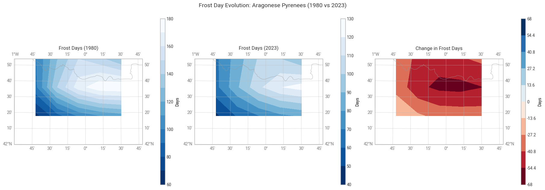
4. Visualizing the “Cold Retreat”
We’ll plot the difference between the two periods to visualize where the decrease in Frost Days is most significant.
[4]:
# Define the Aragonese Pyrenees bounding box [min_lon, max_lon, min_lat, max_lat]
# Adjust these slightly if your specific dataset has different borders
ARAGON_EXTENT = [-1.0, 0.8, 42.0, 42.9]

plot_matrix = [
    [
        ("Frost Days (1980)", fd_80, "Blues_r"),
        ("Frost Days (2023)", fd_23, "Blues_r"),
        ("Change in Frost Days", diff_fd, "RdBu"),  # _r flips it so red = decrease/warming
    ]
]

figure = ekp.Figure(rows=1, columns=3, figsize=(18, 7))

for row_idx, row_plots in enumerate(plot_matrix):
    for col_idx, (name, data, cmap) in enumerate(row_plots):
        # Create map and immediately set the spatial focus
        map_plot = figure.add_map(row=row_idx, column=col_idx, domain=ARAGON_EXTENT)

        # Validate data within the domain
        valid_data = data.values[~np.isnan(data.values)]

        if valid_data.size == 0:
            map_plot.title(f"{name} (No data in domain)")
            continue

        # Logic to center the anomaly colorbar at 0
        if "Change" in name or "Anomaly" in name:
            # Find the maximum absolute deviation from zero
            max_val = np.nanmax(np.abs(valid_data))
            # Create symmetric levels (e.g., from -40 to +40)
            style = ekp.styles.Style(colors=cmap, levels=np.linspace(-max_val, max_val, 11))
        elif np.all(valid_data == valid_data[0]):
            style = ekp.styles.Style(colors=cmap, levels=[valid_data[0] - 1, valid_data[0] + 1])
        else:
            style = ekp.styles.Style(colors=cmap)

        # Plotting & Layers
        map_plot.quickplot(data, style=style)

        # Adding high-resolution features for a small domain
        map_plot.coastlines(resolution="10m", color="black", linewidth=1)
        map_plot.borders(resolution="10m", linestyle="-")  # Helpful for France/Spain border

        # Gridlines with labels restricted to the Pyrenees box
        map_plot.gridlines(draw_labels=True, dms=True)

        map_plot.title(name, fontsize=12)
        map_plot.legend(location="right", label="Days")

# Add a super-title for the entire figure
figure.title("Frost Day Evolution: Aragonese Pyrenees (1980 vs 2023)")
figure.show()