Introduction to Precipitation-based Climate Indices¶

This notebook demonstrates how to compute and visualize precipitation-based climate indices from CMIP6 datasets using the earthkit-climate and xclim packages.

We use:

Precipitation-based indices:
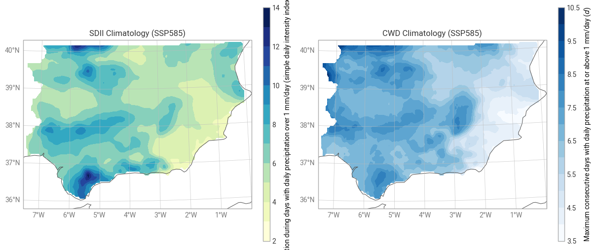
- SDII: Simple Daily Intensity Index (average precipitation on wet days)
- CWD: Consecutive Wet Days (max number of wet days in a row)

We load ACCESS-CM2 CMIP6 data for both historical and SSP585 scenarios.

[3]:

import warnings
from typing import Any, List, Union

import cartopy.crs as ccrs
import earthkit.data as ekd
import earthkit.plots as ekp
import matplotlib.pyplot as plt
import xarray as xr

from earthkit.climate.atmos import precipitation

warnings.filterwarnings("ignore")

plt.rcParams["figure.figsize"] = (8, 5)


def plot_climatology(
    figure: Any, data: xr.DataArray, row: int, col: int, title: str, cmap: Union[str, List[str]], units: str
) -> None:
    """
    Compute and plot the temporal mean of a dataset on a map.

    Parameters
    ----------
    figure : Any
        The figure or layout object where the map will be added.
    data : xarray.DataArray
        The input data containing a 'time' dimension to calculate the climatology.
    row : int
        Row index in the figure grid.
    col : int
        Column index in the figure grid.
    title : str
        Title for the specific map plot.
    cmap : str or list of str
        Color map name or list of colors for the plot style.
    units : str
        Units of the data for styling and legend labeling.

    Returns
    -------
    None
        The function modifies the `figure` object in place and does not return a value.
    """
    # Compute climatology (mean over time)
    climatology: xr.DataArray = data.mean("time")

    # Define style and plot
    # 'ekp' seems to be the library providing the Style and mapping tools
    style = ekp.styles.Style(colors=cmap, units=units)

    # The domain is now explicitly defined within the function
    map_plot = figure.add_map(row=row, column=col, domain=[-7.5, 0, 35.8, 40.2])

    map_plot.quickplot(climatology, style=style)
    map_plot.coastlines()
    map_plot.gridlines()
    map_plot.title(title)
    map_plot.legend(location="right")

Loading CMIP6 data¶

We’ll use daily gridded data from the ACCESS-CM2 model for precipitation (pr), for both historical and SSP585 future scenarios.

[4]:

# Load precipitation
pr_hist = ekd.from_source("earthkit-climate-sample", "pr_ACCESS-CM2_historical_reference").to_xarray()
pr_ssp585 = ekd.from_source("earthkit-climate-sample", "pr_ACCESS-CM2_ssp585_far_future").to_xarray()

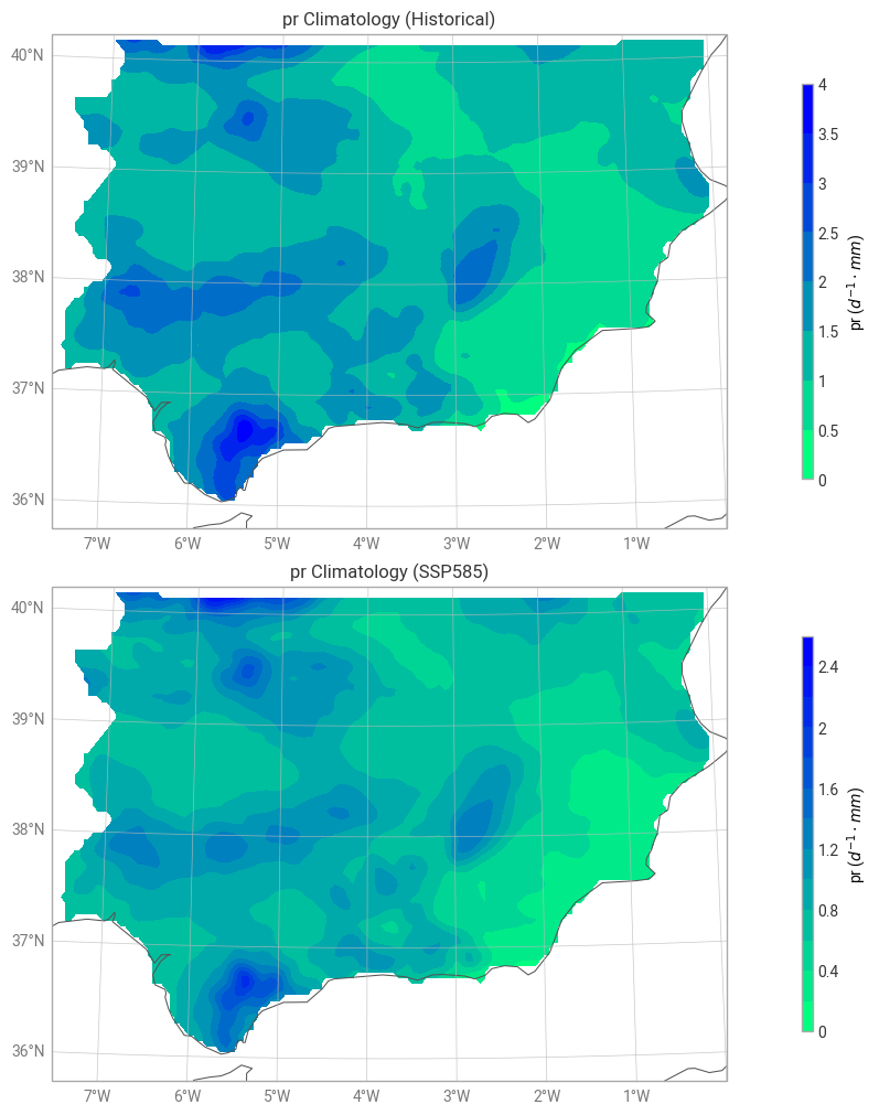
Inspect and visualize the raw data¶

Before computing indices, let’s plot an example grid to see how the raw precipitation looks.

[5]:

# Create the figure with 2x1 maps
figure = ekp.Figure(
    crs=ccrs.NearsidePerspective(central_longitude=-3.75, central_latitude=38.0), rows=2, columns=1, size=(15, 10)
)

# HISTORICAL (row 0)
plot_climatology(figure, pr_hist, 0, 0, "pr Climatology (Historical)", "winter_r", "mm/day")

# SSP585 (row 1)
plot_climatology(figure, pr_ssp585, 1, 0, "pr Climatology (SSP585)", "winter_r", "mm/day")

# Final layout
figure.show()

../_images/how-tos_intro_precipitation_indices_5_0.png

Visualization of Precipitation Indices¶

Let’s visualize the climatologies (average across years) of these precipitation indices.

[8]:

# Create the figure with 1x2 maps
figure = ekp.Figure(
    crs=ccrs.NearsidePerspective(central_longitude=-5, central_latitude=43), rows=1, columns=2, size=(12, 6)
)

# Plot SDII
plot_climatology(figure, sdii, 0, 0, "SDII Climatology (SSP585)", "YlGnBu", "mm d-1")

# Plot CWD
plot_climatology(figure, cwd, 0, 1, "CWD Climatology (SSP585)", "Blues", "days")

# Final layout
figure.show()

../_images/how-tos_intro_precipitation_indices_11_0.png

Introduction to Precipitation-based Climate Indices¶

Loading CMIP6 data¶

Inspect and visualize the raw data¶

Compute Simple Daily Intensity Index (SDII)¶

Compute Consecutive Wet Days (CWD)¶

Visualization of Precipitation Indices¶