Introduction to Temperature-based Climate Indices¶

This notebook demonstrates how to compute and visualize temperature-based climate indices from CMIP6 datasets using the earthkit-climate and xclim packages.

We use:

Temperature-based indices:
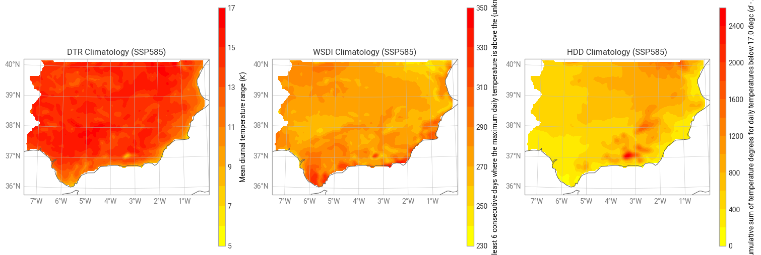
- DTR: Daily Temperature Range (Tmax - Tmin)
- WSDI: Warm Spell Duration Index (≥6 consecutive days above 90th percentile)
- HDD: Heating Degree Days (based on temperature below threshold)

We load ACCESS-CM2 CMIP6 data for both historical and SSP585 scenarios.

[1]:

import warnings
from typing import Any, List, Union

import cartopy.crs as ccrs
import earthkit.data as ekd
import earthkit.plots as ekp
import matplotlib.pyplot as plt
import xarray as xr

from earthkit.climate.atmos import temperature
from earthkit.climate.utils.percentile import calculate_percentile_doy

warnings.filterwarnings("ignore")

plt.rcParams["figure.figsize"] = (8, 5)

Loading CMIP6 data¶

We’ll use daily gridded data from the ACCESS-CM2 model for maximum (tasmax) and minimum (tasmin) temperature, for both historical and SSP585 future scenarios.

[2]:

# Load temperature
tasmin_hist = ekd.from_source("earthkit-climate-sample", "tasmin_ACCESS-CM2_historical_reference").to_xarray()
tasmin_ssp585 = ekd.from_source("earthkit-climate-sample", "tasmin_ACCESS-CM2_ssp585_far_future").to_xarray()

tasmax_hist = ekd.from_source("earthkit-climate-sample", "tasmax_ACCESS-CM2_historical_reference").to_xarray()
tasmax_ssp585 = ekd.from_source("earthkit-climate-sample", "tasmax_ACCESS-CM2_ssp585_far_future").to_xarray()

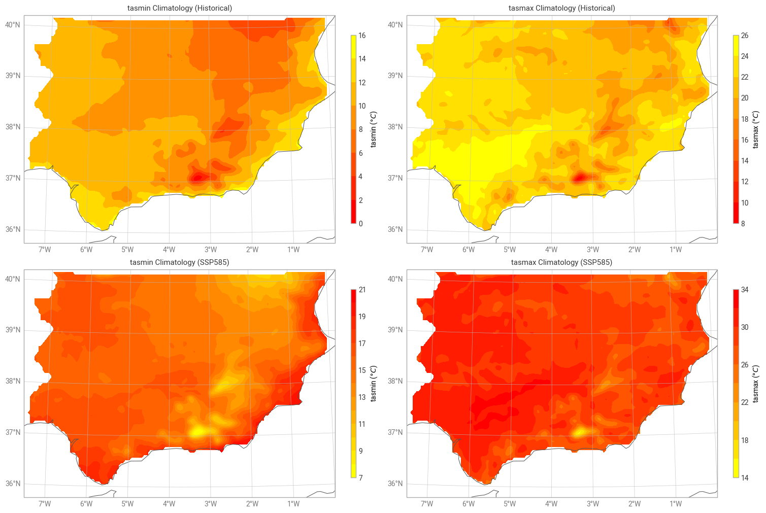
Inspect and visualize the raw data¶

Before computing indices, let’s plot a few example grids to see how the raw variables look.

[3]:

def plot_climatology(
    figure: Any, data: xr.DataArray, row: int, col: int, title: str, colors: Union[str, List[str]], units: str
) -> None:
    """
    Plots a climatological map based on the mean over time.

    Parameters
    ----------
    figure : Any
        The figure object where the map will be added. Typically a
        custom plotting canvas or layout manager.
    data : xarray.DataArray
        The dataset containing atmospheric or oceanic variables.
        Must include a 'time' dimension to calculate the mean.
    row : int
        The row index in the figure layout where the plot will be placed.
    col : int
        The column index in the figure layout where the plot will be placed.
    title : str
        The title text to display above the individual map.
    colors : str or list of str
        The color scale or list of colors to be used by the style engine.
    units : str
        The measurement units for the data (e.g., 'K', 'm/s'), used
        for the style and legend.

    Returns
    -------
    None
    """
    # Se asume que 'domain' está definido globalmente o es accesible
    # en el scope de la función original.
    map_plot = figure.add_map(row=row, column=col, domain=domain)

    style = ekp.styles.Style(colors=colors, units=units)

    # Cálculo de la climatología (media temporal) y graficado
    map_plot.quickplot(data.mean("time"), style=style)

    # Elementos geográficos y estéticos
    map_plot.coastlines()
    map_plot.gridlines()
    map_plot.legend(location="right")
    map_plot.title(title)


# Define domain (Southern Spain)
domain = [-7.5, 0, 35.8, 40.2]

# Create the figure with 2x2 maps
figure = ekp.Figure(
    crs=ccrs.NearsidePerspective(central_longitude=-3.75, central_latitude=38.0), rows=2, columns=2, size=(15, 10)
)

# HISTORICAL
plot_climatology(figure, tasmin_hist, 0, 0, "tasmin Climatology (Historical)", "autumn", "celsius")
plot_climatology(figure, tasmax_hist, 0, 1, "tasmax Climatology (Historical)", "autumn", "celsius")

# SSP585
plot_climatology(figure, tasmin_ssp585, 1, 0, "tasmin Climatology (SSP585)", "autumn_r", "celsius")
plot_climatology(figure, tasmax_ssp585, 1, 1, "tasmax Climatology (SSP585)", "autumn_r", "celsius")

figure.show()

../_images/how-tos_intro_temperature_indices_5_0.png

Visualization of Temperature Indices¶

Finally, let’s visualize the climatologies of these temperature indices across our domain.

[7]:

# Create the figure with 1x3 maps
figure = ekp.Figure(
    crs=ccrs.NearsidePerspective(central_longitude=-3.75, central_latitude=38.0), rows=1, columns=3, size=(15, 6)
)

# PLOT: Each index climatology using the helper function
plot_climatology(figure, dtr, 0, 0, "DTR Climatology (SSP585)", "autumn_r", "K")
plot_climatology(figure, wsdi, 0, 1, "WSDI Climatology (SSP585)", "autumn_r", "days")
plot_climatology(figure, hdd, 0, 2, "HDD Climatology (SSP585)", "autumn_r", "K days")

figure.show()

../_images/how-tos_intro_temperature_indices_13_0.png

Introduction to Temperature-based Climate Indices¶

Loading CMIP6 data¶

Inspect and visualize the raw data¶

Compute Daily Temperature Range (DTR)¶

Compute Warm Spell Duration Index (WSDI)¶

Compute Heating Degree Days (HDD)¶

Visualization of Temperature Indices¶